A quick tour of the GUI

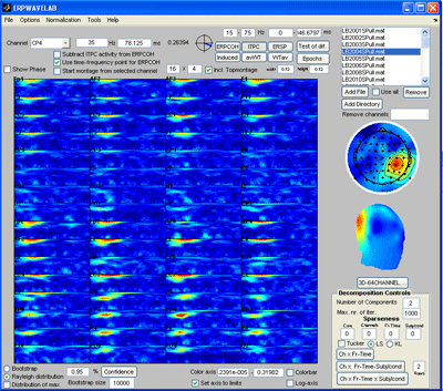
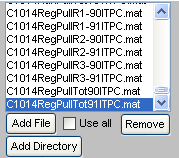
In the upper right area of the user interface the datasets can be loaded and selected for analysis. While ‘Add File’ and ‘Add Directory’ loads a single file and a whole directory respectively, the panel above (named the ‘file browser’) display all the files opened. To remove a selected file simply select the file and push the  ‘Remove’ button. Finally, by selecting ‘Use all’, the grand average over all files of the currently selected  measures is calculated. (To reduce RAM usage only one dataset is loaded into memory at a time.)

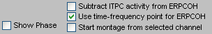
The panel to the left of the ‘file browser’  gives buttons enabling you to
 select the  various measures provided by ERPWAVELAB, see the
 ERPWAVELAB article for details.  By clicking each button
the measure given by the button is calculated and displayed
 in the montage plot and in the Topographical montage plot
 given as a separate figure.  (To calculate linear coherences, select: Options -> Linear Coherence ).

To the right under the montage plot are given various options as to how the current measure is displayed. Right below the montage plot is given the lower and upper value of the currently used color axis. By clicking the ‘Set axis to limits’, the lower value will automatically be set to the minimum value of the current measure and the upper value to the maximum of the current measure in the selected ROI. Finally, a color bar can be displayed by clicking
the  ‘Colorbar’ box and the current measure can
 be log transformed by selecting ‘Log-axis’.

To the left under the montage plot is given various control buttons for accessing significance.  By selecting the confidence level and clicking the ‘Confidence’ button a significance level is calculated and significant regions indicated by red and green contours in the Montage plot (Red marks significantly elevated areas while green contours mark significantly decreased areas).  The confidence interval is two sided for all measures except the ITPC and ERPCOH. While the confidence of the ITPC and ERPCOH can also be estimated by the theoretical Rayleigh distribution of random ITPC and ERPCOH, the significance of all other measures are accessed by bootstrapping, i.e. randomly generating surrogate dataset from a user specified baseline region. Two forms of significance levels are given. One giving the significance of each single data point, the other giving that an activity is significant granted the number of data points present in the montage plot area. This latter form of significance is the distribution of the maximum value of a random dataset containing the same amount of data points as the present dataset displayed (i.e. a conservative correction for multiple comparisons).
Finally, the ’Bootstrap size’ indicates how many
 random samples are generated. Notice, when
‘distribution of max ‘ is selected the very ends
(tails) of the bootstrap samples is considered.
 Thus, a very large bootstrap size is required for this estimation to be valid.

To reduce the region of interest  (ROI) displayed in the
montage plot area change the channel and time range above
these buttons. Below, the buttons containing the various measures, it is possible  to control how the montage plot displays the data, presently as a 16 x 4 array. Furthermore, the width and  height of the time-frequency plot in the topographical  montage given in a  separate figure can also be defined,
presently being plots of size 0.1 x 0.1.

To the left above the
montage plot is given details
of the current channel-
frequency-time point inspected as well as the absolute value and phase of the current measure in this data point given to the right. The activity of each channel at the current time-frequency point is displayed in the topographic  plot area. 

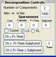
Finally, the control buttons to the lower right of the user interface are available by ERPWAVELAB for the various decomposition techniques. Here the various parameters for the decomposition can be set, i.e. the number of components, maximum number of iterations, sparseness imposed on the various modalities, model type (PARAFAC or TUCKER) and algorithm: ‘LS’ is least  square minimization corresponding to maximizing the variance explained by the model. KL is the Kulback-leibler divergence minimization.

The ‘Ch x Fr-Time’ button decomposes the current measure displayed in the montage plot area into Channel activations for  various time-frequency activities.
The ‘Ch x Fr-Time-Subj/cond’ button decomposes the current measure showing the most commonly activated regions in the scalp as well as giving the specific time-frequency activity in this region for each loaded dataset in the ‘file browser’.
The ‘Ch x Fr-Time x Subj/cond’  button decomposes the current measure showing the most commonly activated scalp region to the most common time-frequency component(s) over various groups of datasets. For details of each of these types of decompositions consult the ERPWAVELAB article.

Montage plot area

Topographic plot area

Underneath the display of the currently
inspected point, various options are given.
‘Start montage from selected channel’,
sets the first channel in  the montage plot to be the currently selected  channel. ‘Use time-frequency point for ERPCOH’  calculates the ERPCOH to all other data  points from the currently inspected data point. Otherwise, the ERPCOH is calculated as the currently inspected channels cross coherence to all other channels within same time and frequency. By selecting  ‘Subtract ITPC activity from ERPCOH’  the ITPC activity is subtracted from the ERPCOH when the ERPCOH is displayed. This enables you to see what activities are more coherent to a given activity than to the event. By selecting ‘Show Phase’ the phase of the current measure (if this measure is complex) is displayed.

Before showing the most common forms of data analysis in ERPWAVELAB a quick overview of the Graphical User Interface (GUI) is given.

Developed by Morten Mørup

A tOOLbox FOR MULTI-CHANNEL TIME-FREQUENCY ANALYSIS